Formulation and In-Vitro Evaluation of Venlafaxine Loaded Polymers Based Nanoparticles

Introduction to Nanoparticles

Nanoparticles (NPs) are nanostructures measuring up to 100 nanometers in all directions. These particles are remarkable in terms of their small size and ability to interact with surface molecules. Because of this, their small particle sizes and huge surface areas change their molecular interactions, opening up new areas of use [1]. The primary factors that dictate the functionality, activity, and utility of the NPs are their properties and structures. For example, the NP's size and shape can affect its optical characteristics, potential for alteration, and ability to enter cells—all of which are critical for uses like imaging research and cancer treatment [2]. Moreover, the NP's surface charge plays a significant role in environmental interaction, impacting not just cellular contact but also the material's properties and potential for toxicity [3]. Assessment of these applications reveals that different kinds of NPs predominate in particular regions. To put it another way, a variety of NP characteristics influence their behavior and cause them to favour particular specialties. The effectiveness and activity of the particle can be greatly altered by the synthesis techniques, size, and shape of the NPs. Taking into account all of these elements, the material selection is also a key determinant of the function, and particularly the kind, of NP. Because of their unique properties, size, and shape, NPs are categorized into three primary types based on the material: inorganic, carbon-based, and organic. They are further differentiated into metallic, ceramic, polymeric, and lipid-based varieties [4]. Recent advancements in biomedical science have led to significant enhancements in the design of therapeutic agents for disease treatment. Nonetheless, a significant challenge to the treatment efficacy of various diseases is the delivery of therapeutic agents to the targeted area. Conventional therapeutic agent’s exhibit limitations, including non-selectivity, adverse side effects, low efficacy, and suboptimal biodistribution. [5, 6]. Thus, design of well-controlled and versatile delivery systems is the main emphasis of present research initiatives. A promising method for delivering a variety of molecules to specific sites in the body is the association of therapeutic medicines with nanoparticles displaying special physicochemical and biological characteristics and structuring their paths for appropriate targeting [7,8]. Targeted therapy in disease treatment involves administering precise quantities of therapeutic agents over an extended duration to the specific area of the body that is affected. The development of safer and more effective therapeutic nanoparticles is essential and represents one of the primary objectives of nanomedicine [8]. Surface modification can also enhance the recognition capability for targeted delivery. Therefore, the cleanability and biodistribution of therapeutic nanoparticles must be carefully considered during the design process. The size of therapeutic nanoparticles is a crucial factor influencing circulation and biodistribution. Nanoparticles measuring less than 10 nm can be efficiently eliminated by physiological systems, such as filtration through the kidneys, whereas particles exceeding 200 nm may be removed by phagocytic cells within the reticuloendothelial system (RES). Therapeutic nanoparticles measuring less than 100 nm exhibit extended circulation times within the bloodstream. Numerous studies have indicated that therapeutic nanoparticles within the size range of 20–200 nm exhibit an increased accumulation rate in tumors, as they are not readily recognized by the reticuloendothelial system and are not filtered by the kidneys[9,10,11]. The surface charge of therapeutic nanoparticles significantly influences their clearance and targeted delivery. Positively charged nanoparticles elicit a more robust immune response in comparison to neutral or negatively charged nanoparticles. Furthermore, nanoparticles exhibiting a surface potential ranging from −10 to +10 mV demonstrate reduced susceptibility to phagocytosis and non-specific interactions [11].

1.2. Introduction To Various Types Of Nanoparticles:

Nanostructure and nanocrystalline are the two primary classifications for nanomaterials. Lipid-based, polymer-based, and non-polymeric nanoparticles are further classifications for nano-structured materials. Dendrimers, nanoparticles, micelles, nanogels, protein nanoparticles, and drug conjugates are examples of polymer-based nanoparticles. Carbon nanotubes, nanodiamonds, metallic nanoparticles, quantum dots, and silica-based nanoparticles are examples of non-polymeric nanoparticles. Liposomes and solid lipid nanoparticles are two types of lipid-based nanoparticles. Most clinically authorized nanoparticles for therapeutic application to date include either lipid-based or polymer-based constituents. Some clinical applications also use nanocrystalline particles, which are created by combining medicinal substances in crystalline form, in addition to polymer-based, non-polymeric, or lipid-based nano-structured particles. [12,13,14,15]

1.3.  Polymer-Based Nano-Particles:

Polymer-based nanoparticles, whether synthetic or natural, offer a viable option for therapeutic applications owing to their biocompatibility, non-immunogenicity, non-toxicity, and biodegradability [16]. To reduce the immunogenicity and toxicity of synthetic polymers such as polycaprolactone (PCL) and polylactic acid (PLA), polyester forms are employed. Conversely, natural polymer-based nanoparticles, including chitosan, gelatin, albumin, and alginate, appear to mitigate toxicity concerns and enhance the efficacy of therapeutic agents relative to traditional approaches. Polymeric nanoparticles are regarded as a matrix system in which the matrix is uniformly distributed. Classification can occur as either Nanocapsules or nanospheres based on their composition. In Nanocapsules, therapeutic agents are enclosed by a distinct polymer membrane, while in nanospheres, these agents are directly dispersed throughout or within the polymer matrix [17,18,19]. The benefits of polymeric nanoparticles as drug carriers encompass their capacity for controlled release, the capability to shield drugs and other biologically active molecules from environmental factors, and the enhancement of bioavailability and therapeutic index [20,21]. The term “nanoparticle” includes both nanocapsules and nanospheres, which vary in their morphology [22]. Nanocapsules consist of an oily core that typically contains the dissolved drug, encased in a polymeric shell that regulates the drug's release from the core. Nanospheres consist of a continuous polymeric network that allows for the retention of the drug either within their structure or adsorbed onto their surface [22,23,24].

1.4. Introduction to Venlafaxine Loaded Polymeric Nanoparticles

Venlafaxine is one of the most potent clinically available serotonin-nor epinephrine reuptake inhibitors (SNRI) antidepressants [25]. It functions by inhibiting serotonin reuptake [26], though its selectivity at the serotonin site is inferior compared to other SSRIs, such as fluvoxamine or sertraline [27]. Venlafaxine is clinically available in oral dosage forms, including tablets, capsules, and oral suspension. It is readily absorbed from the gastrointestinal tract and extensively metabolized in the liver; consequently, a significantly reduced amount of the drug reaches systemic circulation, leading to poor bioavailability. The half-life varies based on dosage and duration of administration. The half-life can extend up to 21 hours after administering a daily oral dose of 30 mgVenlafaxinee [26]. To address these issues, Transdermal patches utilizing solid lipid nanoparticles (SLNs) can be developed to enhance patient comfort; additionally, the formulation of these patches allows for the circumvention of the first-pass effect [27]. Lipid-based nanoparticulate systems have demonstrated significant efficacy in enhancing drug bioavailability. Solid lipid nanoparticles (SLNs) are sub-micron colloidal carriers made up of lipids, fatty acids, waxes, and triglycerides, which are dispersed in an aqueous surfactant solution or water. They are typically considered safe for oral, topical, and parenteral administration [28,29]. Solid lipid nanoparticles (SLNs) are innovative colloidal drug carriers that enhance drug stability, improve drug release profiles, and consequently increase bioavailability and biocompatibility [30, 31]. SLNs systems facilitate safe and effective drug delivery to the target site while minimizing side effects commonly associated with other nanoparticle systems. They serve as alternatives to established nanocarriers such as liposomes, polymeric nanoparticles, and nano-emulsions [32]. Since 1990, solid lipid nanoparticles (SLNs) have been chosen as substitutes for liposomes and polymeric nanoparticles due to their ability to address various issues associated with earlier nanocarrier systems. SLNs are considered safer than polymeric nanoparticles because their production does not involve organic solvents. Additionally, they demonstrate superior drug stability and prolonged release compared to Liposomes [33]. The preparation and evaluation methods for solid lipid nanoparticles (SLNs) are thoroughly documented, and scaling up production is feasible [34].

Polymeric nanoparticles (PNPs) offer several advantages in drug delivery, making them a promising approach for pharmaceutical applications. They enhance bioavailability by improving drug solubility and stability [35,36]. Their controlled and sustained release properties help maintain therapeutic drug levels for extended periods, reducing dosing frequency and improving patient compliance [37,38]. PNPs also enable targeted drug delivery, minimizing systemic side effects and enhancing drug accumulation at the site of action [39,40]. Their biocompatibility and biodegradability make them suitable for long-term applications with minimal toxicity concerns [41,42]. Additionally, their ability to cross biological barriers, such as the blood-brain barrier, expands their use in neurological disorders [43,44]. These advantages highlight the potential of polymeric nanoparticles in modern drug formulation and delivery systems [45].

AIM:

To formulation and in - vitro evaluation of Venlafaxine loaded polymers-based nanoparticles

OBJECTIVES:

Development of polymeric nanoparticles.

In-vitro evaluation of developed polymeric nanoparticles formulation.

MATERIAL AND METHODS

4.1. List of Chemicals and Equipment Used

Venlafaxine and Ethyl Cellulose were purchased from Loba Chemie Pvt. Ltd, Mumbai, and Maharashtra. Tween 80 and organic solvents such as Acetone and Ethanol were purchased from Himedia Laboratories Pvt. Ltd, Thane, and Maharashtra.                  

Table1 1: List of chemicals    

Table2: List of Equipment

4.3. Pre-Formulation Studies

4.3.1. Physio-Chemical Properties

Physical and chemical properties of the Venlafaxine were identified by using different methods, such as colour, nature, form, melting point, pH and odour of the selected drug and the details are recorded.

4.3.2. Bulk Density, Tapped Density, Angle of Repose, Carr’s Index and Hausner’s Ratio

Micromeritic is an imperative subject in pharmaceuticals related to the consideration of small particles and the arrangement of particles measured in microns. The applications of Micromeritic in drug stores are as follows:

• Bulk density helps to evaluate whether the powder has a large bulk volume or not.
• The scattered flow demonstrates no consistency of weight.
• Another flow characteristic of the drug is measured by the angle of repose of the solid drug particles.

4.3.3. Solubility Studies

The solubility of the drug was carried out in various solvents. A small excess quantity (about 25mg) was taken and put into 10ml of each investigated solvent in a 50ml volumetric flask, and the volume made up to the mark. The solubility study was done at room temperature (25°C). The selected drug of a specific amount was added to each conical flask until undissolved particles were observed even after equilibrium for 6 hours with continuous shaking. The supernatant liquid was analyzed using a UV spectrophotometer for the drug dissolved until two successful readings of analysis were constant. The solubility study of Venlafaxine in various solvents is recorded as well as documented [46].

4.3.4. Preparation of Standard Calibration Curve

The standard curve calibration method for a drug involves preparing a series of standard solutions with known concentrations. These solutions are analyzed using an appropriate analytical technique, such as UV spectrophotometry, to measure the corresponding signal response (e.g., absorbance or peak area). The drug was dissolved in a minimal amount of methanol and then diluted with phosphate buffer (pH 6.8) to obtain final concentrations of 5, 10, 15, 20, 25, and 30µg/mL Absorbance for each concentration was recorded spectrophotometrically at 261 nm. The obtained data points were plotted on a graph with concentration on the x-axis and signal response on the y-axis, followed by linear regression analysis to generate a calibration curve [47].

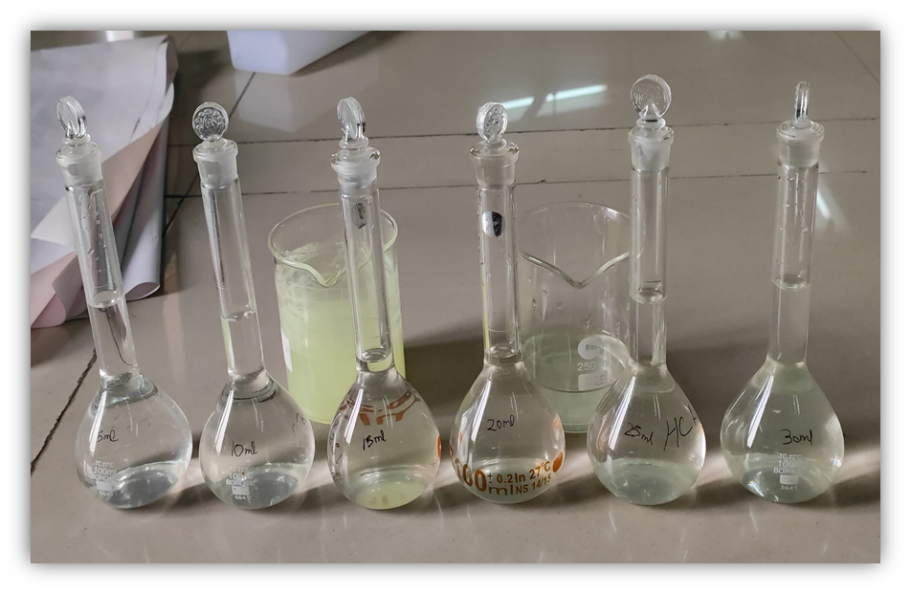
Fig. 5:  Stock Solution of API mixed with PBS Solution

4.5. Fourier Transform Infra-Red (FT-IR) Spectroscopy

4.5.1. FT-IR of Drug (API)

FT-IR spectra were recorded on the sample prepared in KBr disks (2 mg sample in 200 mg KBr disks) using a Broker lab India infrared spectrometer. The drug was scanned over a frequency range of 292 cm?¹.

4.5.2. FT-IR of Drug (API + Excipients)

4.5.2.1 Drug-Excipients Interactions by Fourier Transform Infra-Red (FT-IR) Spectroscopy

The compatibility between the drugs and excipients was compared using FT-IR spectra within a frequency range of 4000-400 cm-1.The position of the peak in the FT-IR spectra of pure Venlafaxine was compared with the FT-IR spectra of Venlafaxine with excipients. It was observed that there was no disappearance or shift in the band position of functional groups in the spectrum of Venlafaxine alone as well as with the excipients. This compatibility study proved that the physical state of Venlafaxine and Venlafaxine with excipients were compatible. Hence, it can be concluded that the drug can be used with the selected polymers without causing instability in the formulation [48].

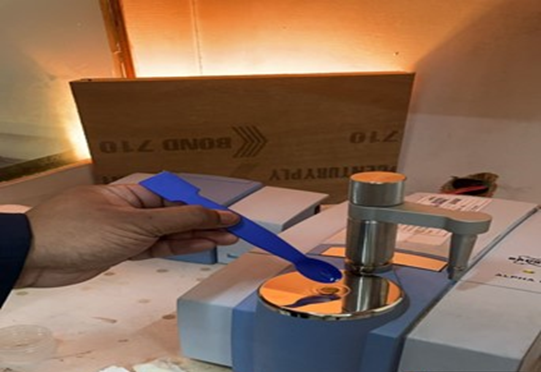
Fig. 6: Image of FT-IR Instrument

4.6. Preparation of Phosphate Buffer

To prepare a phosphate buffer with a pH of 6.8, begin by dissolving approximately 27.21 grams of Potassium Dihydrogen Orthophosphate (KH?PO?) in 1000 milliliters of distilled water. Next, add around 8 grams of Sodium Hydroxide (NaOH). Take 250 milliliters of this solution and pour it into a beaker. Separately, dissolve about 112 milliliters of NaOH in distilled water and add this to the beaker, followed by 250 milliliters of the potassium dihydrogen orthophosphate solution. Add distilled water to bring the total volume to 1000 milliliters. Mix thoroughly. Check the pH of the mixture: if the pH is below 6.8, add more NaOH; if the pH is above 6.8, add HCl until the pH reaches 6.8. The phosphate buffer is ready once the pH is stabilized at 6.8 [49].

4.7. Formulation design

Different batches of Venlafaxine loaded polymeric nanoparticles were prepared based on the 22 Box-Behnken factorial designs. The independent variables were Polymer conjugates concentration in terms of mg (X1) and HPH pressure in terms of bar (X2) with the drug concentration of 20 mg for all formulation batches.

Table3: List of Composition of Formulations

4.7. 1.Preparation of Venlafaxine loaded Polymeric Nanoparticles

Polymeric nanoparticles (PNPs) were formulated via the solvent evaporation process, utilizing Hydroxypropyl methylcellulose (HPMC), ethyl cellulose (EC) and Tween 80 alongside ethanol as the solvent and distilled water for the aqueous phase. Initially, EC was dissolved in ethanol, followed by the addition of HPMC into the same mixture along with the drug. Meanwhile, Tween 80 was integrated into distilled water to form the aqueous phase. EC and HPMC were dissolved in ethanol to form the organic phase, while Tween 80 acted as a stabilizer to augment nanoparticle formation. The organic phase was gradually introduced into the aqueous phase under magnetic stirring for 3 hours to encourage emulsification and ensure uniform distribution of EC and HPMC. Following thorough mixing, the resulting emulsion underwent high-speed homogenization at 15000 rpm for 1 hour to further diminish particle size and enhance homogeneity. Subsequently, the mixture underwent sonication for 30 minutes to break down larger particles and achieve a uniform dispersion of PNPs. Following sonication, the mixture was transferred to a rotary evaporator for solvent evaporation, with the remaining ethanol cautiously eliminated under controlled conditions. The rotary evaporator settings were adjusted from 250 mbar and gradually decreased to 140 mbar over 15 minutes to aid ethanol removal, resulting in the sedimentation of PNPs. After the rotary evaporator process, the suspension was poured into centrifuge tubes and subjected to centrifugation at 15000 rpm for 45 minutes, further resulting in nanoparticles that were filtered through micro porous filter paper. The filtrate was dried using a spray dryer for 20-30 minutes, and the dried NPS were collected [50]

4.7.2. Preparation of Venlafaxine loaded Polymeric Nanoparticles (Steps)

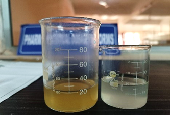
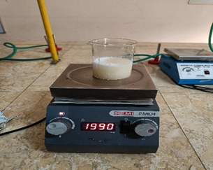
Fig. 8: Magnetic Stirring

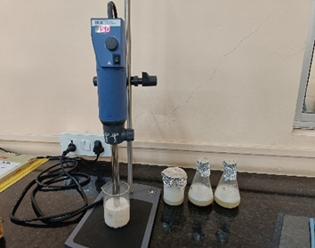
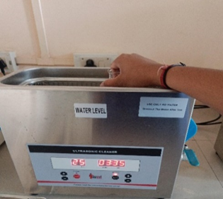
Fig. 10: Sonication

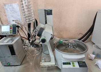
Fig. 12: Centrifugation         

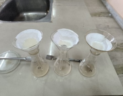
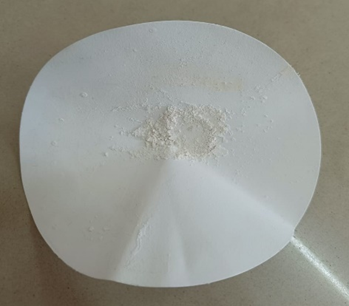
  Fig. 14: Filtrates (NPs

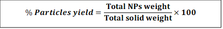
4.8.1. Percentage Yield of Polymeric Nanoparticles

Nanoparticles smaller than 1 micron pass through the filter paper, while aggregates of drug, polymer, and stabilizer are eliminated.The filtrate was subsequently ultracentrifuge at 10,000 rpm for 20 minutes in each batch using a Remi RM-12C micro centrifuge. The supernatant and pellet were separated using a Millipore filter with a pore size of 0.45 µm. The weight of the residue was determined by combining all residues and pellets and weighing them. The weight of nanoparticles was calculated by subtracting the residual weight from the starting weight of solid introduced to the process. The percentage yield of PNPs, also called Nanoparticle recovery, can be calculated using the given equation [51].

4.8.2. Drug Loading

To determine drug loading, the PNPs formulation was centrifuged to separate the dispersed phase from the continuous phase. The supernatant was collected, and the released drug was assayed spectrophotometrically at 261 nm. The precipitate particles were filtered using Whatman filter paper, washed with water, and then accurately weighed. The percentage of drug loading was calculated using an equation [52].

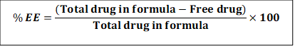
4.8.3. Determination of Entrapment Efficiency (EE) of polymeric nanoparticles

The PNP formulation was centrifuged at 5,000 rpm for 20 minutes. The supernatant solution underwent filtration and separation. After diluting 1 ml of the filtrate with water, the absorbance at 261 nm was measured using a UV spectrophotometer with Phosphate buffer (pH 6.8) as the blank. Then, the amount of free drug in the formulations was assessed to determine the entrapment efficiency. The entrapment efficiency of PNPs can be calculated using the given equation [53].

4.8.4. In-vitroDrug Release Studies

The in-vitro drug release of Venlafaxine -loaded nanoparticles was investigated in Phosphate Buffer Saline (PBS) pH 6.8 solutions utilizing a dissolution test apparatus. 50 mg of nanoparticles were weighed and placed into the capsules. The water level for the environment is maintained, and the temperature is set at 37?C and 80 rpm. The jar was filled with 900ml of PBS, and the sample was removed at regular intervals (5, 10, 15,20,25,30 minutes) and replenished with 5 ml of PBS. The extracted samples were stored in test tubes. After 30 minutes, the samples were checked using UV spectroscopy for the absorbance at 292 nm [54].

4.8.5. Particles Size Analysis:

The Zetasizer (HSA3000) was used to conduct particle size analysis research on the nanoparticulate formulation. The freeze-dried NPs were reconstituted using double-distilled demineralised water. Samples were placed in square glass curettes, and particle size distribution was measured for optimal formulations. The improved formulation was diluted with excess water, and particle size was calculated [55].

4.8.6. Scanning Electron Microscope (SEM)

SEM (ESEM EDAX XL-30) was used to characterize polymeric nanoparticles. Freeze-dried samples were stored in a gold-coated graphite sample container. The chamber was maintained at 0.6 mm Hg pressure and 20 kV voltages. Scanning electron photomicrographs were taken at various magnifications [56].

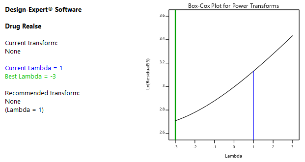
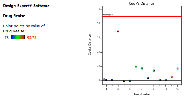
4.8.7. Optimization Data Analysis and Model Validation

ANOVA was used to establish the statistical validation of the polynomial equations generated by Design Expert® Software. Fitting a multiple linear regression model to a 3 2 Factorial design give a predictor equation incorporating interactive and polynomial term to evaluate the responses:

???? = ????0+ ????1????1 +????2????2 + ????12????1????2+ ????11????12 +????22????22 ----Where Y is the measured response associated with each factor level combination; b0 is an intercept representing the arithmetic average of all quantitative outcomes of nine runs; bi (b1, b2, b11, b12 and b22) are regression coefficients computed from the observed experimental values of Y and X1 and X2 are the coded levels of independent variables. The terms X1 X2 represent the interaction terms. Three-dimensional response surface plots resulting from equations were obtained by the Design Expert® software [57].

4.8.8. Kinetic modelling of drug release

The release data were fitted into different mathematical models (Zero-order, First-order, Higuchi, and Korsmeyer-Peppas models) using DD Solver (Excel Add-in) to determine the mechanism of drug release (8,9). The correlation coefficient (R²) values were used to identify the best-fit kinetic model, while the release exponent (n) from the Korsmeyer-Peppas equation was analyzed to determine whether the release followed Fickian or non-Fickian diffusion [58].

RESULT AND DISCUSSION:

5.1. Physical and Chemical Properties of Drug: Venlafaxine

Table: 4: List of Physical and Chemical Properties of Drug:

5.2. Density, Micromeritic and Flow Properties of Drug

Table 5: Density, Micromeritic and Flow Properties of Drug

Its value is in average of three readings.

5.3. Solubility of Drug

Table 6: List for Solubility of Drug and Excipients

5.4. Standard Curve of Drug:

Table:7.  List of Reading of Standard Curve of Drug:

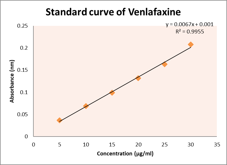
Fig.15: Graph Plot of Standard Curve of Drug

Table: 8. Statistical Parameters

5.5.1. FT-IR of Drug:

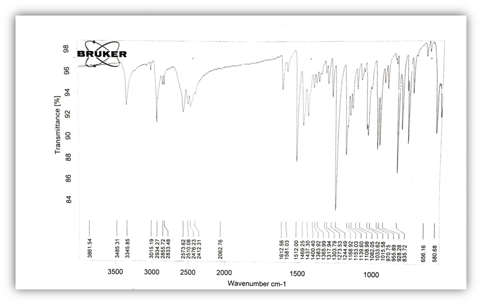
Fig.16: FT-IR of Drug:

5.5.2. FT-IR of Drug-Excipients Interaction:

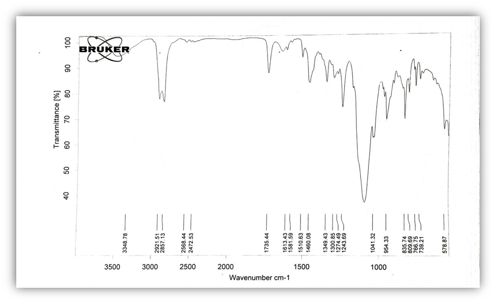
Fig.17: FT-IR of Drug with Excipients

Table.9:  FT-IR Peak of Functional Groups of drug and excipients:

FTIR analysis was performed to assess the compatibility of the drug with excipients in the nanoparticle formulation. The characteristic peaks of the pure drug were compared with those of the drug-excipients mixture to detect any significant shifts. The results confirm that no major chemical interactions or degradation occurred, demonstrating the suitability of the excipients for nanoparticle formulation.

5.6. Percentage Yield of the Prepared Polymeric Nanoparticles:

Table 10: List of Percentage Yield of the Prepared Polymeric Nanoparticles:

All the batches showed production yield in between 66 to 85%. The resultant yield is an indication that the method can be appropriate for technology transfer that is production on large scale. The optimized batch showed production yield was found to be 84.33%.

5.7. Percentage Drug Loading:

Table 11. List of percentage Drug Loading:

All the batches showed drug loading in between 11to 28%. The resultant drug loading is an indication that the method can be appropriate for technology transfer that is production on large scale. The optimized batch showed drug loading was found to be 22.21%.

5.8. Percentage Entrapment Efficiency of Prepared Polymeric Nanoparticles:

Table12. List of Percentage Entrapment efficiency of Prepared Polymeric Nanoparticles:

All the batches showed entrapment efficiency in between 66-90%. The resultant entrapment efficiency is an indication that the method can be appropriate for technology transfer that is production on large scale. The optimized batch showed entrapment efficiency was found to be 89.23%.

5.9. In-vitro Drug Released Studies of Prepared PNPs

Table13. List for % Drug Release of F1, F2, F3, F4, F5 and F6 Formulation:

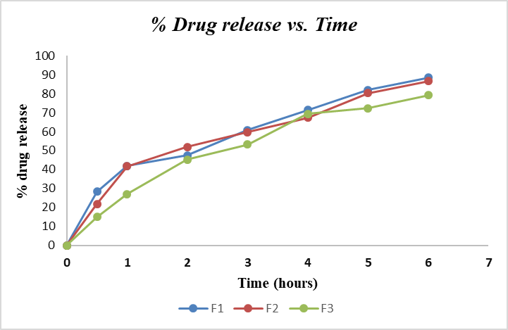
Fig.18: Graph Plot of In-vitro Drug Release of Formulation F1, F2 and F3

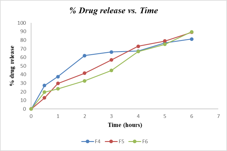
Fig.19: Graph Plot of In-vitro Drug Release of Formulation F4, F5 and F6

Table 14. List of In-vitro % Drug Release of F7, F8, F9, F10, F11 and F12 Formulation:

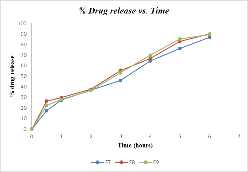
Fig.20: Graph Plot of In-vitro Drug Release of F7, F8and F9 Formulation

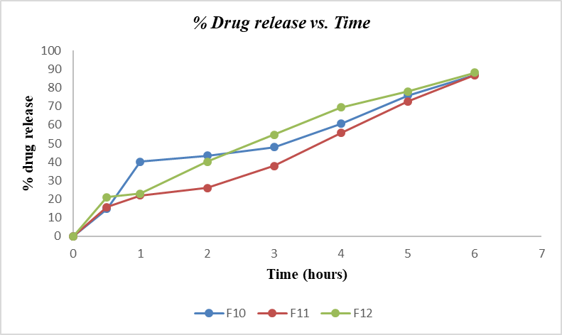
Fig.21: Graph Plot of In-vitro Drug Release of F10, F11 and F12 Formulation

In-vitro drug release profiles of Venlafaxine loaded NPs were obtained by dissolution test apparatus Electro lab in phosphate buffer solution (pH 6.8). NPs filled capsules were placed in a capsule shaker and sealed. This is immersed into 900ml phosphate buffer solutions and the system was maintained 37°C under agitation of 85rpm/min. Aliquots were collected for every 30 mints up to 210 mints and the same was replaced with fresh buffer. The samples were further analyzed using UV-Spectrophotometer and absorbance was measured 292nm. Venlafaxine loaded NPs batch F7 showed 91.53% The expected characteristics of NPs of sustained released was verified.

5.10. In-vitro Drug Release Kinetics:

The in-vitro drug release kinetics of the optimized formulations was analyzed using the software named “DD Solver”. The results were highlighted in bold values and indicate that the Korsmeyer-Peppas model provided the best fit for the formulations F7. This suggests that the release mechanism follows a combination of diffusion and erosion processes, consistent with the characteristics of the Korsmeyer-Peppas model.

Table 15. List of the in-vitro Kinetics Models:

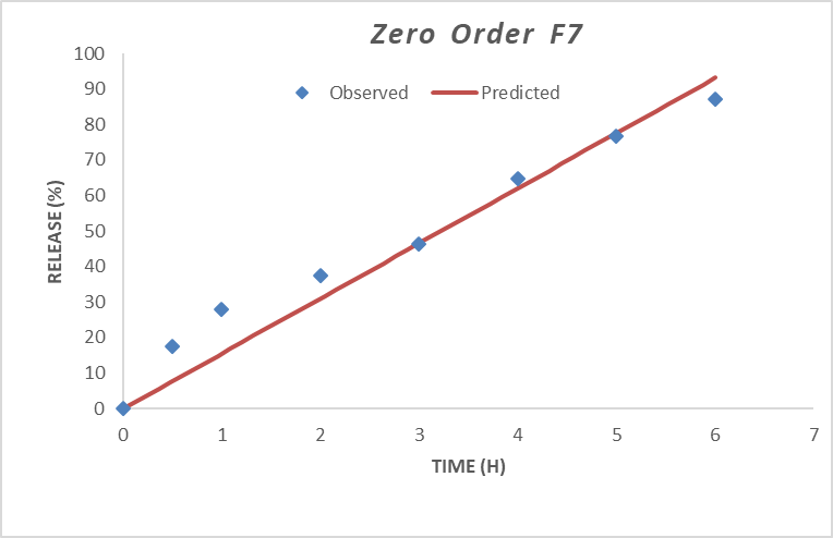
Figure 22. Graph Plot of In-vitro Kinetics Model using DD Solver for F7

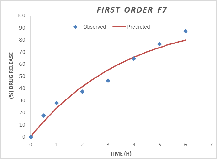
Fig.22: Graph Plot of In-vitro Kinetics Model using DD Solver for F7:

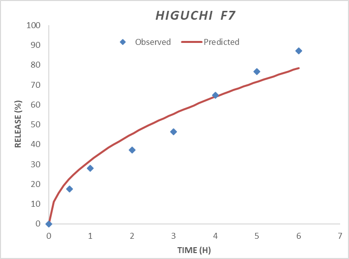
Fig.23: Graph Plot of In-vitro Kinetics Model using DD Solver for F7:

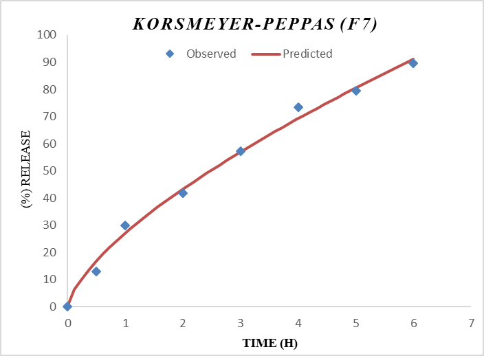
Fig.24: Graph Plot of In-vitro Kinetics Model using DD Solver for F7:

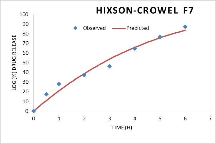
Fig.25: Graph Plot of In-vitro Kinetics Model using DD Solver for F7:

5.11. Particles Size Analysis:

Table 16. List of the Particles Size:

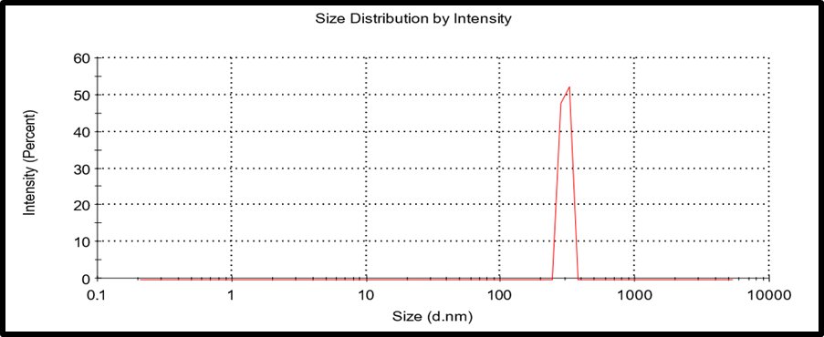
Fig.26: Images of Particles Size of F7:

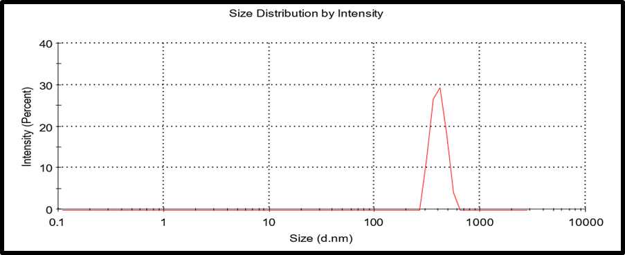
Fig.27: Images of Particles Size of F7:

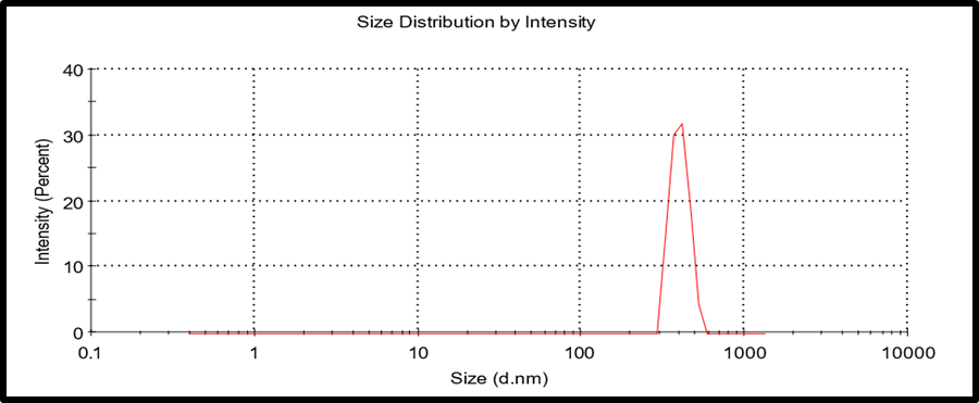
Fig.28: Images of Particles Size of F7:

In addition to its ability to control the pace and degree of drug release and absorption, the particle size of the PNs is a crucial issue. The bioavailability of the medicine is enhanced by the smaller particle size, which provides a greater interfacial surface area. Among all the twelve prepared formulation, the particles size (PS), poly dispensability Index (PDI) of the F7 was considered as the best formulation with particles size to be found 366,386,398nm and PDI values was found to be 0.44,0.74,0.85. The average particles size of the formulation F7 was considered to be 383.33, as considered the best formulation.

5.12. Scanning electron microscope (SEM):

Based on formulation optimization, including % yield, drug loading, entrapment efficiency, and in-vitro drug release experiments, the F7 formulation was shown to be consistent and optimal. As a result, the F7 formulation was studied using Scanning Electron Microscopy (SEM) to determine the surface shape of the polymeric nanoparticles. The SEM image indicated that the nanoparticles of the Formulation F7 were smooth and spherical in structure. This nanoscale size confirms the successful formation of polymeric nanoparticles, which is a critical prerequisite of achieving enhanced drug bioavailability and therapeutic efficacy.

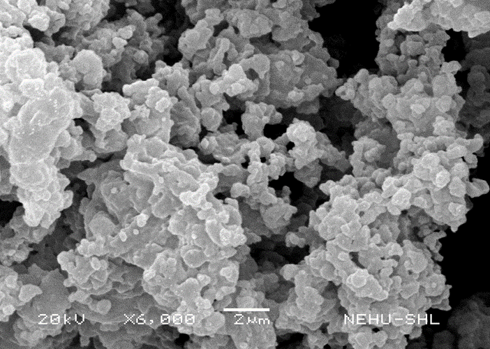
Fig.29:  Images of SEM of Polymeric Nanoparticles of F7

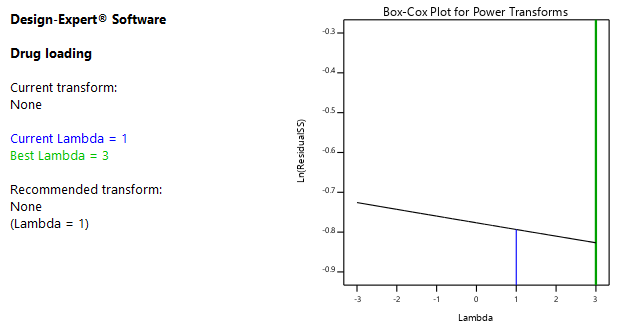
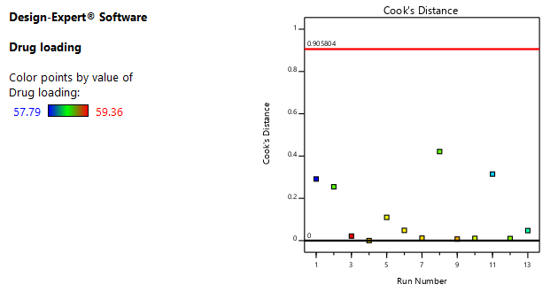
5.13. Fitting of Data and Model

Independent variables demonstrate that the model was significant for all the response variables. It was observed that independent variables X1 (polymer concentration) and X2 (HPH pressure) had a positive effect on the entrapment efficiency and drug loading of the nano-formulation that was nanoparticles was achieved. The statistical evaluation was performed by using ANOVA. The results were showed in below table. The coefficients in the regression equation that contain more than one factor term are called interaction terms. This demonstrates that the link between variables and responses is not necessarily linear. When more than one element is changed at the same time and at various levels in a formulation, the reactions might vary.

5.13.1. Fit Summary

Response 1: Drug loading

Table 17: Model Comparison for Drug Loading Prediction

Table 18: Sequential Model Sum of Squares [Type I]

ANOVA for Linear model

Response 1: Drug loading

Table 19: ANOVA Summary for Linear Predicting Drug Loading

Fit Statistics

ANOVA for Linear model:

Table 20: Fit Statistics for Drug Loading Prediction Model

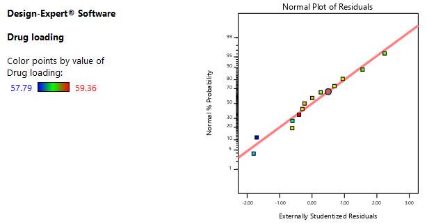
5.13.2. Fit Summary

Fig. 30: Images of ANOVA Linear Model for Drug Loading

Response 2: Drug release                            

Table 22: Model Comparison for Drug Loading Prediction

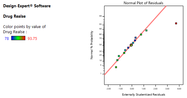
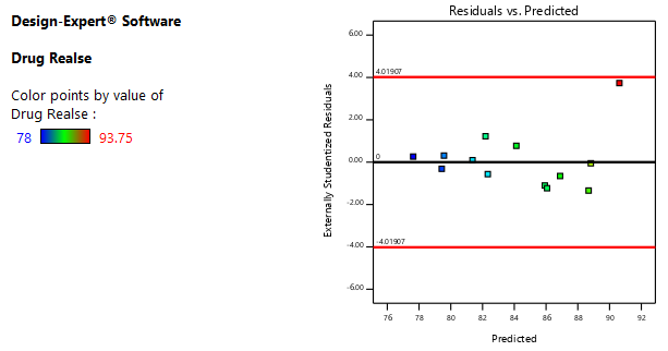
Response 2: Drug Release

Table 23: ANOVA Summary for Linear Model Predicting    

Fig.31: Images of ANOVA Linear Model for Drug Release

5.14.3D surface plot analysis:

Three-dimensional surface plots were generated by the Design Expert® software are presented in (Figure no. Fig.32 and Figure no. Fig.33 for the studied responses, i.e. Mean Drug loading (Y1) and Entrapment Efficiency (Y2). Fig.32 depicts response surface plot of Polymer Conjugate Concentration (X1) and HPH Pressure (X2) on Mean of Drug loading. Nanoparticles being nanoparticulate structures, formulation batch amongst all the design batches giving least particle size will be preferred more and selected as an optimized batch. Where F7 Design Batch, with a polymer concentration of about 150mg and 200mg, show the least particles size i.e. 383.33nm. Fig.33 depicts response surface plot of Polymer Conjugate Concentration (X1) and HPH Pressure (X2) on entrapment efficiency. The 3-D surface image shows a linear response, which indicates with the increase in the polymer concentration the entrapment efficiency increases, as more the polymer available more will be the entrapment efficiency. Here, two design batches i.e. F2 and F7 showed maximum entrapment efficiency i.e. 81.73% and 89.23% respectively. But as seen in first response Surface graph being a nanoparticle formulation considering the least particle size is also a crucial factor. So, the Design Batch with least particle size and maximum entrapment efficiency is selected. Therefore, F7 is considered as an optimized Batch.

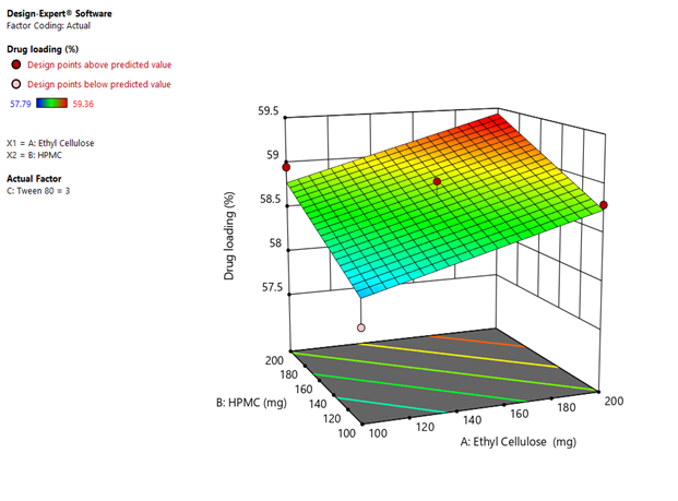
Fig. 32: 3D surface Plot for X1 and X2 on drug loading, where X1= Polymer conjugates concentration and X2 = HPH pressure

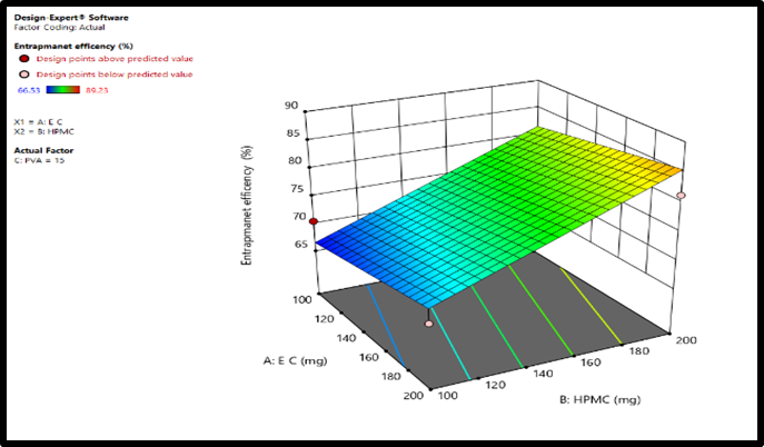
Fig. 33: 3D surface Plot for X1 and X2 on drug release, where X1= Polymer conjugates concentration and X2 = HPH pressure

REFERENCES

Parbati Kumari Shah*, Pankaj Chasta, Dr. Peeyush Jain, Formulation and In-Vitro Evaluation of Venlafaxine Loaded Polymers Based Nanoparticles, Int. J. of Pharm. Sci., 2025, Vol 3, Issue 3, 191-218. https://doi.org/10.5281/zenodo.14968465
10.5281/zenodo.14968465