Mathematical Modeling of Two-Phase Non-Newtonian Blood Flow by Power Law in the Renal Artery with Hemodynamic Analysis of Dengue Patient

RENAL BLOOD VESSEL ^[1,2,3,4]

Renal Vascular Anatomy

Terminal End-Arteries: The intrarenal arterial system consists of end-arteries characterized by a complete absence of parenchymal anastomoses. Consequently, occlusion of any branch inevitably leads to localized tissue infarction. Dual Capillary Beds: The renal vasculature features a distinct portal-like architecture consisting of two sequentially arranged capillary networks: Glomerular Capillaries: A high-pressure network optimized exclusively for ultrafiltration. Peritubular Capillaries: A low-pressure network optimized for solute reabsorption and gas exchange around the tubular segments. Filtration Hemodynamics: The high-pressure state within the glomerular capillaries is precisely regulated by the structural resistance of both the afferent and efferent arterioles, which serve as the primary pre- and post-capillary control gates for the Glomerular Filtration Rate (GFR).

Renal Blood Flow (RBF) Dynamics

Perfusion Volume: The kidneys receive a disproportionately large share of the cardiac output (20–25%, equivalent to ~1000 mL/min or 400 mL/100g/min).

Intrarenal Perfusion Gradient:

Cortex: Receives 95% of total RBF to maximize filtration capacity. Medulla: Receives a restrictive 5% of total RBF. This low-velocity perfusion is a physiological necessity to prevent the washout of the hypertonic medullary urea gradient, thereby preserving the countercurrent mechanism required for urine concentration. Metabolic Paradox: The massive blood supply to the kidneys is driven by functional filtration demands rather than metabolic consumption. Consequently, the renal fractional oxygen extraction is exceptionally low (10–15%, consuming roughly 4 mL/100g/min).

Oxygen Dissociation Stability: Renal oxygen extraction remains remarkably constant despite fluctuations in RBF. This is because renal metabolic oxygen expenditure is directly proportional to GFR and the subsequent energetic workload of tubular sodium reabsorption. [Alex Yartsev 2020]

Macro-Anatomy of the Main Renal Trunk^[5,6,7,8]

Aortic Origin and Dimensions: Each kidney is perfused by a primary renal artery, a major large-bore muscular branch arising directly from the abdominal aorta. Morphologically, these vessels typically span 4–5 cm in length and 5–10 mm in diameter, frequently demonstrating a slight physiological asymmetry in caliber between the left and right sides. Pre-Parenchymal Bifurcation: Immediately prior to penetrating the renal parenchyma, the main trunk bifurcates into distinct anterior and posterior main branches. These primary divisions subsequently branch into segmental arteries before entering the dense tissue of the organ.

Micro-Anatomy & Intrarenal Perfusion Architecture

Absolute End-Artery Architecture: Beyond the segmental transition, the intrarenal arterial tree maintains a strict end-artery configuration characterized by an absolute absence of collateral vascular networks or intra-parenchymal anastomoses (Bertram, 2000). Territorial Vulnerability to Ischemia: Because there are no secondary back-up connections between adjacent arterial segments, the occlusion or hypoperfusion of any single segmental branch leads directly to isolated, regional ischemia confined strictly to its specific anatomical territory of distribution.

The normal Peak Systolic Velocity (PSV) for a healthy main renal artery is between 60 and 150 cm/s. The End-Diastolic Velocity (EDV), which measures blood speed at the end of a heartbeat, normally ranges from 20 to 50 cm/s. The Renal-Aortic Ratio (RAR) is the renal artery velocity divided by the abdominal aorta velocity, with a normal value under 3.5. The Resistive Index (RI), indicating resistance within kidney tissue, typically falls between 0.50 and 0.70. Acceleration Time (AT), the time for blood to reach peak flow, should be less than 70 milliseconds. Abnormal diagnostic criteria -PSV exceeding 180 to 200 cm/s, suggesting kidney artery narrowing. RAR of 3.5 or more, indicating severe renal artery stenosis (>60% blockage).RI above 0.70, which implies intrinsic kidney damage or medical renal disease rather than artery blockage.AT delayed beyond 70 to 80 milliseconds, showing upstream blood flow restriction before reaching the kidney^[12].

2. DENGUE DISEASE^[13]

Dengue Fever (DF):This is the classic form of dengue where blood vessels remain stable. Hematocrit (Hct): Normal or slightly elevated. Any minor rise is due to mild dehydration from high fever. Blood Pressure (BP): Normal. The circulatory system functions perfectly fine, keeping readings near 120/80 mmHg.

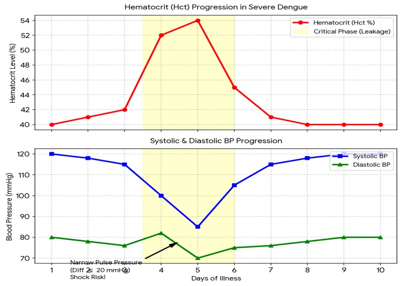
Dengue Hemorrhagic Fever (DHF)Microscopic holes develop in blood vessels, causing the liquid part of blood (plasma) to leak out. Hematocrit (Hct): Rises significantly ( 20% increase). As plasma leaks, the blood becomes severely thick. A baseline Hct of 40% will spike to 48% or higher. Blood Pressure (BP): Systolic drops and Diastolic rises. The top number drops from fluid loss. The bottom number rises as blood vessels squeeze to compensate. This creates a narrow reading like 100/80 mmHg.

Dengue Shock Syndrome (DSS):This is a medical emergency where the circulatory system crashes completely. Hematocrit (Hct): Either spikes critically or drops catastrophically. It peaks very high from extreme plasma loss, but it will suddenly crash to very low levels if severe internal bleeding occurs. Blood Pressure (BP): Severe Hypotension. The blood pressure drops completely. The gap between the top and bottom numbers narrows to 20 mmHg or less (e.g., 80/65 mmHg). In deep shock, it becomes unrecordable.

Febrile Phase (Days 1 to 3)Hematocrit: Remains baseline flat near 40%.Blood Pressure: Stable and wide apart (e.g., 120/80 mmHg), indicating a strong and healthy circulatory volume. Critical Phase & Shock Risk (Days 4 to 6)Hematocrit Spikes: Plasma leaks out of the vessels, causing the hematocrit curve to shoot upward sharply above 50%.BP Line Convergence: The top (systolic) line plummets due to severe volume loss, while the bottom (diastolic) line temporarily rises or stays firm due to vascular constriction. The gap between them constricts to 20 mmHg or less, signaling Dengue Shock Syndrome. Convalescence/ Recovery Phase (Days 7 to 10) Hematocrit Normalizes: The body naturally reabsorbs fluids, causing the blood thickness to dilute back down to a safe 40%. BP Stabilizes: The systolic and diastolic lines pull apart to a healthy, wide gap, normalizing blood circulation.

3. TWO PHASES OF BLOOD ^[14]

Blood exhibits remarkable non-Newtonian character when Several researchers studied the blood flow characteristics in the presence of stenoses in the lumen of the arteries (Ikbal et al., 2009; Sankar, 2010; Ismail et al., 2008). Blood behaves like a Newtonian fluid when it flows in larger diameter arteries at high shear rates. Many studies were carried out to analyze the steady and unsteady flow of blood in larger diameter arteries, treating it as Newtonian fluid (Liu et al., 2004; Chakravarty and Mandal, 2004; Sud and Sekhon, 1985). Blood exhibits remarkable non-Newtonian character when it flows through narrow diameter arteries at low shear rates and blood flow in narrow arteries is highly pulsatile, particularly in diseased state.

Low Shear Rate (< 100 s⁻¹) — Pure Non-Newtonian Behavior

This occurs when blood flows very slowly, such as in tiny capillaries, branching microvessels, or during the resting phase of the heart (diastole). At this low force, Red Blood Cells (RBCs) begin to aggregate and stick together, stacking like a pile of coins. This physical structure is called a Rouleaux formation. This crowding makes the blood highly viscous (thick). Because its viscosity changes with force, blood exhibits a specific Non-Newtonian trait known as Shear-Thinning (Pseudoplastic) behavior.

High Shear Rate (100 s⁻¹ to 200 s⁻¹) — Newtonian Transition

This occurs when blood moves at a high velocity through large blood vessels, such as the aorta or major arteries. The high fluid forces completely break apart the Rouleaux cell clusters. The individual red blood cells stretch out and align perfectly parallel to the direction of the flow. Once the shear rate crosses 100 to 200 s⁻¹, the viscosity levels off and becomes virtually constant (asymptotic). At this point, blood behaves mathematically as a standard Newtonian fluid. Since here the strain rate of renal artery is 12 to 37.5 so blood is showing a non-Newtonian behavior[15]. 

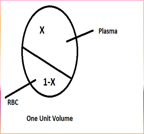
In this case blood divided into two phase by unit volume fluid.

4. REAL MODEL

4.1Parametrization

The blood's velocity 

 and any two thermodynamic quantities related to it, such as pressure, 

 and density, 

),were distributed according to functions that affected the mathematical description of the state of a moving blood. All thermodynamic quantities, together with the equation of state, are determined by the values of any two of them, as is often known. Thus, we may fully ascertain the condition of flowing blood if we have five variables: the density ρ , the pressure P, and the three components of velocity vk.

The coordinates 

, and the time t are functions of all these values. It stressed that the blood's velocity at a given position

 in space and at a given time t was represented by the expression

.

Flow pattern of two phase blood flow in artery vessel ^[16,17]

In our two phases of blood assumption

Let one unit volume of whole blood and

X= volume fraction of plasma

Y= 1-X

 volume fraction of RBC

the mass ratio of RBC  to plasma is m

where 

 are the densities of RBC,plasma.

we define density of blood mixture ρm

 as follows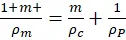

         

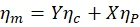
And viscosity of blood mixture ηm as follows

4.2 Boundary conditions.

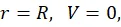
1. The velocity of blood flow on the axis of blood vessels at r = 0 will be maximum and finite, say v0= maximum velocity.

2. The velocity of blood flow on the wall of blood vessels at r = R, where, R is the radius of blood vessels, will be zero. This condition is well known as no slip condition.

4.3 Equation of Continuity

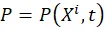
continuity equation for three  phases

         [1]

          [2]

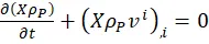
Where, vi is the common velocity of two phase blood cells and plasma. Again Xρcvi,i

 is co-variant derivative of (Xρcvi)

 with respect to Xi.

Equation of motion for blood flow with the three phases using the principle of force conservation (or momentum conservation) in hepatic arteries and assuming that the consistency coefficient (or viscosity coefficient) of RBC cells is ηc.

Yρc∂vi∂t+Yρcviv,ji-YP,jgij+Yηcgjkvi,k,j

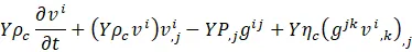
Similarly, taking the viscosity coefficient of plasma to be the equation of motion for plasma will be as follows-

XρP∂vi∂t+XρPviv,ji-XP,jgij+XηPgjkvi,k,j

then equation of motion for blood flow with the all three  phases will be as follows-

ρm∂vi∂t+ρmvj vi,j =-P,jgij+ηmgjkvi,k,j

  [3]

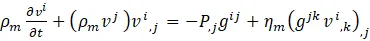
Whenever percentage of blood is reduces the blood has been supposed Newtonian but in case of increasing the hematocrit, the effective viscosity of blood flowing through arteries remote from the heart depends on the strain rate.

For this reason,the blood will flow as non Newtonian fluid. When strain rate is in between 5 to 200 per second, the power law

τ'=ηmen

where 0.68≤𝑛 ≤0.80 Describes the flow of blood very well. The constitutive equation of blood is as follow

Blood's constitutive equation is as follows:

τij=-pgij+ηm(eij)n=-pgij+τ,ij

       [4]

Where τij

 is stress tensor and τ,ij

 is shearing stress tensor.

4.4 Mathematical formulation

The equation of continuity for power law flow will be as follows:

1g(gvi),i=0     

                       [5]

Again the equation in tensorial form is as follows:

ρm∂vi∂t+ρmvjvi,j=τij,j   

[6]

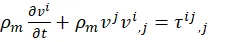
Since the blood vessels are cylindrical, the above governing equation have to transformed into cylindrical co-ordinates.

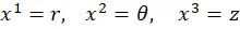
Let x1=r,    x2=θ,     x3=z

Matrix of corresponding  metric tensor in cylindrical form is as follow:

gij=1000r20001

So Matrix of conjugate metric tensor is

gij=10001r20001

Where as Christoffel’s symbols of 2^nd kind are as follows:

122=-r,   221= 212= 1r

     except of these all are zero.

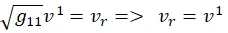
Contravarient and physical components of velocity of blood flow will be related as

g11v1=vr=>  vr=v1

 g22v2=vθ=> vθ= rv2,

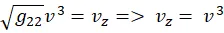
g22v3=vz=> vz= v3

Further the physical component of -p,jgij are-giip,jgij

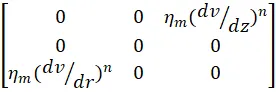
The matrix of physical component of shearing stress – tensor

τ,ij =ηm(eij)n=ηm(gikv,ki+gjkv,kj)n

  [7]

will be as follows :

00ηm(dvdz)n000ηm(dvdr)n00

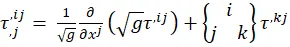
The covariant derivative of τ,ij

 is

τ,j,ij= 1g∂∂xjgτ,ij+ijkτ,kj

      [8]

Keeping in view the above facts the governing tensorial equation can be transformed  into cylindrical form which are as follows :

The Equation of continuity –

∂v∂z=0

The Equation of motion –

r

-Component                                          

-∂p∂r=0

θ

-Component

0=0

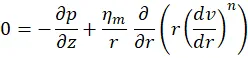
Z-Component

0=-∂p∂z+ηmr ∂∂rrdvdrn

These are the r

, θ,z

   components respectively

Further the fact has been considered  that  axial flow in artery is symmetric, so that  vθ=0 and vr ,  vz  and p

 do not depend upon θ

. Also the blood flows steadily,i.e.

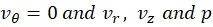
∂p∂t=∂vr∂t=∂vθ∂t=∂vz∂t=0

On integrating equation,we get vz=vr

 because  v does not depend upon θ

 

The integration of equation of motion, we get p=pz

 since p does not depend upon θ

   

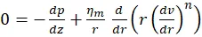
Now, with the help of equation, the equation of motion  converts in the following form:

0=-dpdz+ηmr ddrrdvdrn

           [9]

The pressure gradient -(dpdz)=P

 of blood flow in the arteries remote from liver can be supposed to be constant and hence the equation  takes the following form:

ddrrdvdrn=- Prηm

On integrating equation (9), we get

rdvdrn=-Pr22ηm+A

       [10]

We know that the velocity of blood flow on the axis of the cylindrical arteries is maximum and constant. So that the apply the boundary condition at r=0, v = V0(

contant), on equation (10) to get the arbitrary constant  A = 0. Hence the equation (10) takes the following form :

-dvdr=Pr2ηm1n

                [11]

Integrating equation  once again, we get

v=-P2ηm1n r1n+1(n+1)n+B

             [12]

To determine the arbitrary constant B, we apply the no –slip condition n the inner wall of the arteries :  at r=R,   V=0,

 where   R=

 radius of vessel, on equation (12) so as to get

B=P2ηm1n nR1n+1n+1

Hence the equation  takes the following form:

v=P2ηm1n nn+1R1n+1-r1n+1

        [13 ]

Which determines the velocity of blood flow in the arteries remote from the liver where P is gradient of blood pressure and ηm

  is the viscosity of blood mixture.

Shear stress  

τ=Q1+3nπnnrηmR3n+1

Strain rate  

dvdr=∆Pr2∆z ηm1n

The total flow- flux of blood through the transverse section of the arteries is

Q=0Rv.2πr dr=0RP2ηm1n.1n+1R1n+1-r1n+12πr dr

  

=P2ηm1n.2πnn+1R1n+1.r22-n.r1n+33n+10R

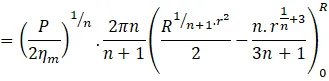
=P2ηm1n.2πnn+1.n+1R1n+323n+1

 

Q= P2ηm1n.πnR1n+33n+1 ,    where P= -dpdz

Q=Pi-Pf2ηm(zi-zf)1n.πnR1n+33n+1

           [14]

5. RESULT & DISCUSSION

Table (a): Pathological Data of Dengue Patient

DAY	Hgb	HCT	B.P (mmHg)	Pressure drop (∆p)
1	13.40	40.2	113/66	23.5
2	13.82	41.46	110/67	21.5
3	14.01	42.03	109/69	20
4	14.03	42.09	106/71	17.5
5	14.25	42.75	105/72	16.5
6	14.40	43.2	103/73	15
7	14.16	42.48	103/73	15

Equation of viscosity

ηm=Yηc+XηP

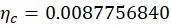
0.0045=ηc42.03100+0.00141-0.4203

ηc=0.0087756840

 pascal sec

Let,H = 42.03

ΔP=Pi-Pf=2457.08 pascal

According to Glenn Elert (2010)

ηm =

 viscosity of mixture = 0.0045  pascal sec

According to Gustafson, Daniel R. (1980)

ηp=

 Viscosity of plasma =0.0014 pascal sec

ηm=Y×ηc+XηP

where Y=H100

ηm=H100×ηc+(1-H100)ηP

ηm=0.0087756840H100+0.00141-H100

 

ηm=7.37×10-5 H+0.0014

Q=660[18]mlmin=1.1×10-5 m3/sec

radius R=0.00375 meter

length of renal artery Δz=0.05 meter

Q=Pi-Pf2ηmzi-zf1n.πn R1n+33n+1

By Newton-Raphson method find value of n

def get_newton_raphson(x):

fx = log(x) - log(1+(3*x)) + (4.311238036/x) - 1.822421518

fx_prime= (1/x)-3/(1+(3*x))-(4.311238036/x**2)

delta = fx/fx_prime

x_new = x - delta

return x_new, delta

def get_optimized_value(x_init, n_iteration, eps):

 for i in range(n_iteration):

   try:

   x_new, delta = get_newton_raphson(x_init)

     print(x_new)

          temp = x_new

          if abs(delta)<=eps:

             n_iteration = i+1

             break

           x_init = x_new

       except:

           x_new = x_init

           n_interation = i

print(f"wrong initial guess: getting x_new = {temp} at {n_interation} iteration")

       break

abs_per_error = abs((x_new-x_init)/x_new)

return x_new, n_iteration, abs_per_error

if __name__=="__main__":

    x_init = 1

    n_interation = 2000

    eps = 0.00000000001

1.464576690641444

1.759308823795298

1.8173835235248155

1.817008976812434

1.8170238619375374

1.817023273466403

1.8170232967359778

1.8170232958158503

1.8170232958522339

1.8170232958507955

x: 1.8170232958507955, n: 10, abs_per_error: 7.916271376316284e-13

here we will take absolute value

n=1.81702329

Further find a mathematical relation between pressure drop and hematocrit

∆P=40.2327 H+764.25

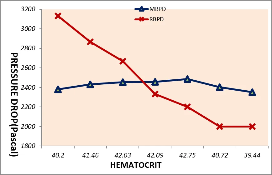
Table (B): Modulated Blood Pressure Drop

DAY	HCT	Modulated BPD (pascal)	Real Clinical BPD (pascal)
1	40.2	2381.57	3133.25
2	41.46	2432.26	2866.59
3	42.03	2455.20	2666.6
4	42.09	2457.61	2333.27
5	42.75	2484.16	2199.94
6	40.72	2402.52	1999.95
7	39.44	2351.02	1999.95

TABLE (c)  r/R v/s shear stress

r/R	STRESS
0	0
0.1	0.0672
0.2	0.1744
0.3	0.3027
0.4	0.4564
0.5	0.3914
0.6	0.8542
0.7	1.105
0.8	1.402
0.9	1.733
1	2.102

Table (d) radius v/s velocity

RADIUS	VELOCITY
0	0.7569
0.005	0.7318
0.001	0.6834
0.0015	0.619
0.002	0.5416
0.0025	0.4526
0.003	0.3532
0.0035	0.2442
0.004	0.1263
0.0045	0

Table (e) radius v/s strain rate

Radius	Strain Rate
0.0025	188.7
0.0027	196.87
0.0029	204.76
0.0031	212.42
0.0033	219.86
0.0035	227.09
0.0037	234.14
0.0039	241.03

Table (f) p-value table

Variable	Mean	SD	P-value
Modulated BPD	2423.48	47.22	0.847
Real clinical BPD	2457.08	441.25	0.847
HCT	41.24	1.17	-

Statistical Interpretation:

The paired t-test showed a p-value = 0.847.Since p > 0.05, there is no statistically significant difference between Modulated BPD and Real Clinical BPD values.

6. CONCLUSION

The comprehensive hemodynamic investigation presented in this study yields several key findings: Because the calculated strain rate of the renal artery falls within  limit (<100 per sec ) blood deviates from Newtonian properties and operates strictly under non-Newtonian power-law behavior. Applying the Newton-Raphson algorithm accurately identifies the characteristic fluid flow behavior index as n=1.81702329 under the prescribed physiological constraints. The progression of Dengue directly elevates blood hematocrit over the course of the illness, peaking around day 5 to 6. This spike thickens the blood mixture, alters effective fluid viscosity, and causes significant deviations between modulated and real clinical pressure drops. Fluid velocity peaks perfectly along the center axis (r=0) and terminates at zero on the arterial wall due to the no-slip boundary condition. Conversely, shear stress exhibits an inverse relationship, rising to its maximum profile of (2.102) at the vessel wall interface (r/R = 1).here value of hct is rising to till 5 days so in these days we will decrease  the drug dose and after we will increase the drug dose rapidly. Overall, this mathematical approach provides a quantitative tool for clinicians to evaluate internal organ perfusion drops and circulatory risks using simple, routine blood test markers like hematocrit.

REFERENCES

1. Just, Armin. "Mechanisms of renal blood flow autoregulation: dynamics and contributions." American Journal of Physiology-Regulatory, Integrative and Comparative Physiology 292.1 (2007): R1-R17.
2. Stein, Jay H. "Regulation of the renal circulation." Kidney international 38.4 (1990): 571-576.
3. Bertram, John F. "Structure of the renal circulation." Advances in Organ Biology Volume 9, 2000, Pages 1-16 (2000)
4. Kriz, Wilhelm, and Brigitte Kaissling. "Structural organization of the mammalian kidney." The kidney: physiology and pathophysiology 3 (1992): 587-654.
5. Braam B., Yip S., Cupples W.A. (2014) Anatomy, Physiology, and Pathophysiology of Renal Circulation. In: Lanzer P. (eds) PanVascular Medicine. Springer, Berlin, Heidelberg. https://doi.org/10.1007/978-3-642-37393-0_146-1
6. Bergström, J., H. Bucht, and B. Josephson. "Determination of the Renal Blood Flow in Man-By Means of Radioactive Diodrast and Renal Vein Catheterization." Scandinavian journal of clinical and laboratory investigation 11.1 (1959): 71-81.
7. Hansell, Peter, et al. "Determinants of kidney oxygen consumption and their relationship to tissue oxygen tension in diabetes and hypertension." Clinical and Experimental Pharmacology and Physiology 40.2 (2013): 123-137.
8. Epstein, Franklin H. "Oxygen and renal metabolism." Kidney international 51.2 (1997): 381-385.
9. Leichtweiss, H-P., et al. "The oxygen supply of the rat kidney: Measurements of intrarenal pO 2." Pflügers Archiv 309.4 (1969): 328-349.
10. Levy, Matthew N. "Effect of variations of blood flow on renal oxygen extraction." American Journal of Physiology-Legacy Content 199.1 (1960): 13-18.
11. Burke, Marilyn, et al. "Molecular mechanisms of renal blood flow autoregulation." Current vascular pharmacology 12.6 (2014): 845-858.
12. Lukas M. Trunz; Rashmi Balasubramanya.Doppler Renal Assessment, Protocols, and Interpretation (2023).
13. Dengue guidelines, for diagnosis, treatment, prevention and control,WHO (2009).
14. Shankar D.S. ‘Journal of Applied Fluid Mechanics’, Vol. 8, No. 4, pp. 871-883, (2014)
15. Alexander Fuchs ‘Assessment of Rheological Models Applied to Blood Flow in Human Thoracic Aorta’;Bioengineering (Basel). 2023 Oct 24;10(11):1240.
16. Pedro-Cabrales-2/publication/230742468/figure/fig7/AS:643939556139011@1530538562826/Two-phase-flow-of-blood-in-a-cross-section-of-an-arteriole-with-a-cell-free-layer-and-red_Q640.
17. Pedro-Cabrales2/publication/230742468/figure/fig1/AS:486125111386114@1492912666595/Cross-section-of-an-arteriole-The-version-of-the-Krogh-tissue-cylinder-model-used-in-our.png
18. Samuel Dambreville, MS ‘Renal Arterial Blood Flow Measurement by Breath-held MRI: Accuracy in Phantom Scans and Reproducibility in Healthy Subjects’Magn Reson Med. 2010 Apr;63(4):940–950.

REFERENCES

Bhaskar Pandey, V. Upadhyay, Mathematical Modeling of Two-Phase Non-Newtonian Blood Flow by Power Law in the Renal Artery with Hemodynamic Analysis of Dengue Patient, Int. J. of Pharm. Sci., 2026, Vol 4, Issue 6, 2854-2866. https://doi.org/10.5281/zenodo.20636279
10.5281/zenodo.20636279